- Meditation on Valuation
- Posts
- Post 2 - A Brief History of Financial Theory
Post 2 - A Brief History of Financial Theory
Part 2 - The Gaussian Cosa Nostra
Drew Miles
September 12, 2023

Paul Samuelson, MIT
Bachelier’s ideas led to some interesting conclusions. MIT’s Paul Samuelson, “The Father of Modern Economics,” was completely bought into the random walk idea. Bachelier, in combination with Eugine Fama’s work on the Efficient Market Hypothesis, inspired him to write this now-infamous quote:
“A respect for evidence compels me to incline toward the hypothesis that most portfolio decision makers should go out of business – take up plumbing, teach Greek, or help produce the annual GNP by serving as corporate executives. Even if this advice to drop dead is good advice, it is obviously not counsel that will be eagerly followed. Few people will commit suicide without a push.”
Samuelson (clearly) vehemently agreed with Bachelier and EMH’s conclusion that no one could beat the market; anyone who does beat the market just got lucky. In fact, the math and logic behind these theories will it to be true. (EMH simply states that the prices of securities or assets at any moment in time are “correct” because they take into account all relevant and up-to-date information. The ultimate conclusion of this theory is that it is impossible to beat the market; no arbitrage opportunities exist. It is very similar and compatible with Bachelier’s ideas.)
Now, I’m not exactly sure how I would handle the discovery of that information, but telling portfolio managers to go kill themselves sure is one way to go about it. But, in Samuelson’s defense, he was not entirely close-minded on this issue. He also wrote:
“It is not ordained in heaven, or by the second law of thermodynamics that a small group of intelligent and informed investors cannot achieve higher mean portfolio return with lower average variabilities.” (i.e. beat the market)
Samuelson just wasn’t convinced that anyone like this existed. There are plenty of examples then and now that back up this claim. Here is a fun one:
From July 2000 through May 2001, a friendly competition involving three groups of professional and amateur investors was run in a fun test of Samuelson’s ideas. Group A, after three arduous rounds of analyses and modeling to try and predict which tech stocks were going to rebound after the Dot Com crash, actually outperformed the market: +4.4% vs the MSCI Europe (their benchmark) which sat at -17%. Group B did not fare as well; they ended the competition down over 80%. Group C did the best; they were up 13.3% after the three rounds, significantly outperforming the market and their other two peer groups. So who were the professionals and who were the amateurs?
Group A were the professionals, if you couldn’t tell from their sophisticated analyses. Group B, the worst performing group, was the amateurs. That must settle the debate, right? Skill looks like it really is a differentiator. Maybe luck has much less to do with successful investing than Samuelson & Co. would imply. That would be a fair conclusion to make until you realize that Group C, the best-performing lot of the bunch, consisted of a single entity: a blindfolded monkey.
The Gaussian Cosa Nostra
Let’s call Samuelson and the other proponents of this random walk/EMH framework the Gaussian Mafia Cosa Nostra. The Cosa Nostra name originates from the now sizable conglomerate of similar thinkers, many of whom have received a Nobel prize. The group includes the likes of Louis Bachelier, Harry Markowitz, William Sharpe, Fischer Black, Myron Scholes, and Robert Merton. Let’s introduce those who are a part of this Cosa Nostra (that we haven’t spent time with yet) one by one and discuss, briefly, the foundations of each; a tour back through business school if you will.
Modern Portfolio Theory

Harry Markowitz, UC San Diego Today
Harry Markowitz was on the hunt for his doctoral thesis when the idea dawned on him. He was reading Theory of Investment Value by John Burr Williams, a book that argued that a stock’s value is simply forecasting the dividends it will pay while adjusting that prediction for inflation, foregone interest, and other uncertainty. Markowitz realized this theory only covered one half of the risk-reward coin (the reward). The risk, Markowitz gathered, is how variable that prediction is relative to other securities’ price movements. Without considering the risk, you would simply invest everything you have in your highest-expected prediction. Not many people think this way in reality, as one naturally considers that their prediction has some chance of being incorrect. So, Markowitz developed relatively simple equations to account for both risk and reward, birthing Modern Portfolio Theory.
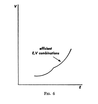
An Efficient Frontier, Portfolio Selection
Markowitz’s theory begins from the premise that there are two steps in the formation of a portfolio. The first is “the formation of the relevant beliefs on the basis of observation” and the second is the actual selection of the portfolio (his paper is aptly named given it only covers the second step).
His theory only takes into account two numbers: the mean and the variance of a certain security’s price movements. If you were to add securities to a portfolio, the weighted average (weighted on the size of your capital stack allocated to each security) of their expected returns and variances would be the expected return and variance of the portfolio. This is just a fancy way of saying, if you have a security that returns 10% on average, and one that returns 12% on average, a 50/50 portfolio consisting of those two securities would result in an expected return of 11% (the same calculation is done for the variance of the portfolio). Of course, some securities tend to move in tandem or opposite of one another. The covariance, a measure of how correlated any two securities’ price movements are, has to be considered as well.
His main trick is to consider diversification via mixing uncorrelated assets in a portfolio together. That way, you may sacrifice some return, but you also reduce the variance, or risk, of a basket of securities (a portfolio). It is the financial equivalent of not putting all your eggs in one basket.
The mathematical framework underlying Markowitz is the same that underlies Bachelier. Remember: Bachelier’s thesis implies the use of a Gaussian, or normal distribution, to describe the mean and variance of price movements. So does Markowitz’s theory. More specifically, it relies on the premise that there are observable and static means (expected values, or averages) and variances of said price movements. It makes the math much cleaner and easier. But Markowitz’s theory wasn’t perfectly easy quite yet.
In order to calculate your expected return, you must calculate a covariance between each and every security you add to your portfolio. That means a 30-stock portfolio would require almost 500 calculations to complete. Not to mention the covariance moves every second the market is open, given prices are constantly changing. And, of course, you must have accurate predictions of expected (mean) returns and variations. Is your mean return how much a firm’s earnings will grow in the next 5 years? Maybe 10 years? Or maybe it’s how much its stock has historically returned or varied over time. But how much time? Nonetheless, this form of security analysis/portfolio management was the beginning of the modern portfolio theory revolution, and it took off.
Capital Asset Pricing Model

William Sharpe, Wikipedia
Markowitz published Portfolio Selection in 1952 and subsequently moved from Chicago to Los Angeles to work at the think-tank RAND Corp. William Sharpe, a struggling doctoral student at UCLA, knocked on Markowitz’s door in 1960. He was a fan of Markowitz’s work and needed help coming up with a thesis idea (the one he was working on was not going well and was advised to drop it entirely). Markowitz had the perfect idea: He wanted Sharpe to simplify Modern Portfolio Theory into a more user-friendly formula. Preferably one that didn’t require endless calculation.
So, Sharpe asked himself what would happen if everyone invested using Markowitz’s ideas. He imagined there was a group of investors with the same goal but invested in different portfolios. One of those investors would be invested in “the right one” i.e., the one with the largest expected return and lowest variance. The other investors would realize this and subsequently move their money into that same portfolio. This ideal portfolio would eventually be known as “the market portfolio.” This was the birth of the index fund.
Because of this conclusion, Sharpe was also able to drive home the point “[An investor] may obtain a higher expected rate of return on his holdings only by incurring additional risk (as defined by the “typical” variation (standard deviation) from the expected return).” This is a conclusion widely held by the investment community still to this day. It is represented by the Capital Market Line below.

Capital Markets Line, Capital Asset Prices: A Theory of Market Equilibrium Under Conditions of Risk
So, if an efficient market comes to realize that only the market portfolio matters, then it was Sharpe’s conclusion that every security should simply be valued relative to the rest of the market. A stock’s expected return would then be defined as the risk-free rate plus the “equity risk premium” multiplied by how sensitive the stock is in relation to the market (Beta).

To define the terms:
· The risk-free rate (Rf) is the rate of return on the safest asset on the planet, usually defined as the yield on a US treasury bond.
· The equity risk premium (E(Rm) – Rf) is the rate of return you expect in excess of the risk-free rate, and is demanded by all rational investors (you would not take on a riskier bet that was paying you 3% per year on your money if the 10-yr US treasury bond was returning, say, 4% each year).
· Beta (β) is how sensitive a stock’s price is relative to the market. When the market goes up 1% and the stock goes up 2%, that implies a beta of 2. If the market goes up 1% and the stock goes down 2%, that implies a beta of -2.
· E(Ri) is then the expected return of this investment.
Sharpe’s formula makes Markowitz’s calculations much, much easier. Rather than calculating how each and every security correlates with each other, you only have to calculate how each security moves with the market, or Beta. The almost 500 calculations needed for a 30-stock portfolio now reduces to 31 (a forecast for the market + 30 betas). Sharpe called his formula the Capital Asset Pricing Model (CAPM).
Sharpe’s theory not only applies to the valuation of assets from an external perspective, it also can be applied within a company that is deciding whether or not to pursue a new project/investment (entire corporate finance courses in business school are dedicated to this topic, none that I’ve found better than Aswath Damodaran’s at NYU). CAPM allows one to judge the “hurdle rate” required for a company to accept or reject a project. If the cost of capital of the firm, as defined by CAPM, exceeds the expected return of a project/investment (say, building a new factory), then it should be rejected. If it does not, then it should be accepted (the factory should be built). This is the essence of all corporate decision-making.
Of course, there are questions to be asked just like with Markowitz’s theory. How exactly should we define “the market”? Again, what time frame should we use if we are defining expected return and risk (mean & standard deviation) when using past data? How often should we recalculate our expected return? Despite these questions, CAPM also exploded onto the scene.
In 1999, a study out of Duke confirmed that ~74% of CFOs use CAPM to estimate their cost of capital. A similar study done in 2015 by MIT estimates that this number could be upwards of 90% today. Of course, there is art in determining which inputs you use in the CAPM formula; those questions mentioned in the previous paragraph can have subjective answers to something that perhaps shouldn’t be so subjective. Getting your hurdle rate (cost of capital) wrong and then making investment decisions based on that is a great way to destroy value.
The final Nobel Laureates in our recap of financial history, the three amigos who defined the Black-Scholes formula for valuing derivatives, deserve special attention. They will be the topic of the next post.
The Opposition
Not all economists and mathematicians bought into the ideas underlying these revolutionary financial theories. But the Cosa Nostra was powerful; dissenting views, like the one written in the mid-1980’s by Robert Fano claiming that the market wasn’t as random as people were claiming, were quickly shot down. “Unless you’re working in a certain way, with certain views, you’re wrong,” he later described.

Beniot Mandelbrot, Yale
Even Benoit Mandelbrot, who is most famous for the recognizable Mandelbrot set of fractals, was offering alternate theories throughout the time that this Cosa Nostra was gaining power and influence in the economics community. He argues that the assumptions that have to be made are too steep of an ask for the theories to work in reality - In order to conclude that price movements follow a random walk, or via Brownian motion, pattern, three key assumptions have to be made:
· Independence: A security’s price changes over time are independent of each other. A stock's next price movement is always 50/50 up or down.
· Gauss: A security’s price movements follow a bell curve. There are lots of small changes, a few big changes, and no extreme changes.
· Stationarity: The process of generating those price changes remains the same. The game never changes.
But we still use all of these theories, so surely these assumptions can’t be that big of leaps, right? Mandelbrot tested these many times, but here is one example that hits on all three:
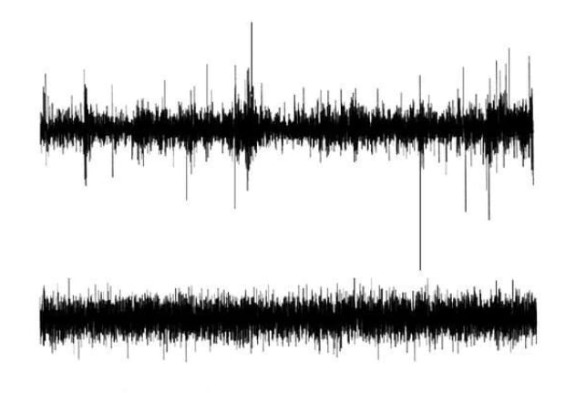
The (Mis)behavior of Markets, Benoit Mandelbrot
Above are charts of two securities’ relative price movements from 1959 - 1996. Clearly, they are not the same. One shows jagged and extreme price movements, while the other depicts a much-less-volatile security. One’s volatility is clustered (the bigger spikes up and down seem to be on top of each other) while the other’s is not. One certainly seems like a much riskier investment than the other.
So, who are the companies? Well, they’re actually the same. The chart on the top is IBM’s relative price changes from 1959 – 1996. The second chart shows how those price movements are supposed to look given random walk’s assumptions. The real chart challenges the three key assumptions made by the Cosa Nostra:
· Independence: The clustering of volatility in the real price chart implies, perhaps, that volatility begets volatility. If true, independence would not hold.
· Gauss: The biggest jumps in price are much larger than anything we see in the random walk simulation. The normal distribution would not allow for this to occur.
· Stationarity: The time period from 1959 to 1996 encompasses the beginning of the Vietnam War and the invention of the internet. Are we sure this game we call investing hadn’t changed over that time period?
Nonetheless, random-walk-based theories became the guiding dogma, and, much to Mandelbrot’s chagrin, Bachelier’s thesis became the premier idea underlying the tools used in modern finance.
Mandelbrot, before his death, called modern finance “a house built on sand.”
Thank you for reading.
Reply